Building an Outbound Reporting Pipeline

Sending email reports with custom, user-specific charts is an easy-sounding, backend engineering task that inevitably becomes a nightmare to maintain. Solutions typically involve cron jobs or manually configured queues and workers, which are brittle, hard to test, and even harder to fix when they fail.

Of course, it doesn’t have to be this way. Data engineering patterns map cleanly to orchestrating user emails and make these straightforward to build.

So today, we’re using Dagster—along with DuckDB, Pandas, Matplotlib and Seaborn—to build an almost production-ready email pipeline. More specifically, we’ll build a monthly revenue report email for hosts of MyVacation, a pretend Airbnb-like company, and tap into Dagster's powerful partitioning features.

What we’re building

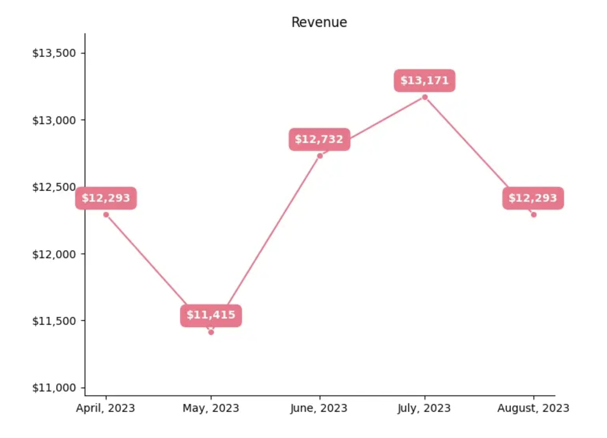
We’re building a tiny version of an email report delivery pipeline. It will calculate an owner’s monthly revenue numbers and create an image containing a line chart with their historical revenue data. This information will then be emailed to the property owners. We’ll work with partition mappings to segment data and resources to connect to remote services. The chart will look like this:

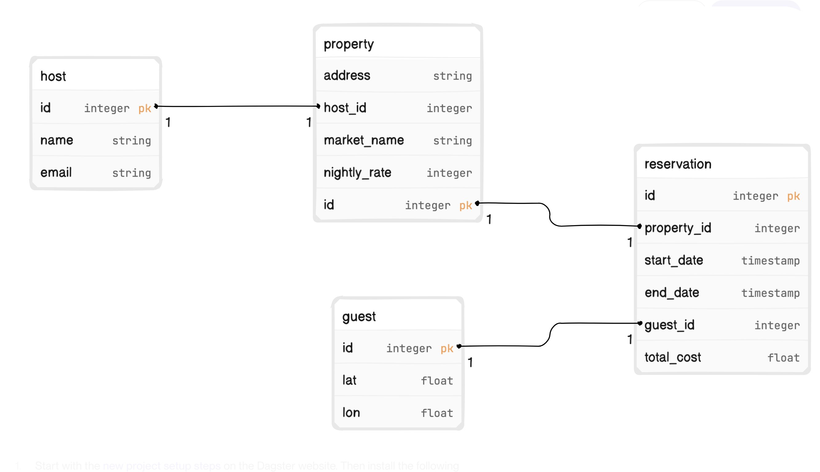
MyVacation is unique in that its application database has only four tables, all of which are necessary for sending a monthly property revenue email.

In our model, guests make reservations at properties which hosts own. Conveniently, all columns are also relevant to the monthly property report email.

Setup

If you’d like to follow along:

1. Start with the new project setup steps on the Dagster website. Then install the following packages:
2. Install dependencies - pip install dagster-duckdb~=0.20 dagster-duckdb-pandas~=0.20 seaborn~=0.12 Faker~=19.2 geopy~=2.3
3. Go to the project’s GitHub and copy the database.py file into your local directory. Running that file will create myvacation.duckdb . We’ll use this as a local application server and back the DuckDB I/O Manager.
4. If you want to create sample data, copy and execute the sample_data.py file
5. Configure your I/O Manager.

# __init__.py

from dagster_duckdb_pandas import DuckDBPandasIOManager

database_io_manager = DuckDBPandasIOManager(database="myvacation.duckdb", schema="main")

defs = Definitions(
        ...
    resources={
        "io_manager": database_io_manager,
         ...
    },
)

Denormalizing Reservation Data

Our first task is combining reservation data with property and guest data to start our analysis, filtering only for reservations completed in the last month.

We’ll use a Partition class to isolate the time range we want to operate on. MonthlyPartitionsDefinition is a predefined partition type that lets us run assets on a month’s worth of reservations. The start and end times for the current partition are available inside the asset’s context object, which we’ll get back to momentarily.

# assets.py

from dagster import MonthlyPartitionsDefinition

@asset(
    partitions_def=MonthlyPartitionsDefinition(start_date="2023-03-01")
)
def monthly_reservations(
    context: AssetExecutionContext
) -> pd.DataFrame:
    bounds = context.partition_time_window
    print(bounds.start)
    print(bounds.end)

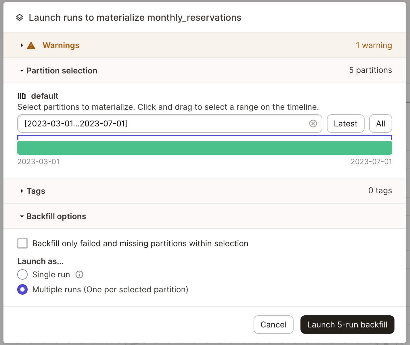
When materializing a partitioned asset in the UI, the available time range is now split up across multiple partitions, where they can be executed individually or in bulk.

Now that our asset has information about the time range, we need to access the database. We could connect directly to a database client, but this approach makes testing and configuration across environments difficult.

Instead, we’ll use another Dagster class to define a configurable database resource that gets passed into our object at runtime.

Database is a simple class that connects to DuckDB and returns a query as a Pandas DataFrame.

# resources.py
from dagster import ConfigurableResource
import duckdb

class Database(ConfigurableResource):
    path: str

    def query(self, body: str):
        with duckdb.connect(self.path) as conn:
            return conn.query(body).to_df()

To make Database available to our asset, define it as a resource in our project’s Definitions object.

# __init__.py
from .resources import Database

...

defs = Definitions(
        ...
    resources={
        "database": Database(path="myvacation.duckdb"),
    },
)

Now if we add database to our function signature, Dagster can pass in our newly created resource.

# assets.py

from .resources import Database
...
@asset(
    partitions_def=monthly_partition_def,
)
def monthly_reservations(
    context: AssetExecutionContext, database: Database
) -> pd.DataFrame:

Thanks to our Database resource, the query results are already converted to a DataFrame when they get back our asset. But they aren’t ready to be returned from our asset yet. The magic of assets is that the results are saved (materialized) and available to downstream assets or ops, even if executed at different times. When configuring our io_manager, we told Dagster to save results by default in DuckDB. So when monthly_reservations returns a DataFrame, Dagster adds the results to a monthly_reservations table in the database. When new partitions are executed, the results are added to the same monthly_reservations table.

This raises a DuckDB-specific question. If the next downstream asset, which depends on the monthly_reservations asset, is also partitioned by month, how does Dagster know which records from the monthly_reservations table need to be made available?

The monthly_reservations asset needs to tell Dagster by specifying which column of its output columns should be used for partitioning via the partition_expr metadata value.

#assets.py

@asset(
    partitions_def=monthly_partition_def,
    metadata={"partition_expr": "month_end"},
)
def monthly_reservations(
    context: AssetExecutionContext, database: Database
) -> pd.DataFrame:

        ...
        results["month_end"] = pd.to_datetime(bounds.end)
    return results

We’re adding a new column that indicates the very end of month that the reservations occurred (technically, it is midnight on the start of the next month), and telling Dagster that this value is a reliable way to determine which partition a record belongs to.

Aggregating Monthly Property Results

Next, we need to calculate how much each property makes per month. We won’t go into detail about this asset because, although it’s important to the pipeline, there are no new concepts other than a Pandas aggregate function.

Since property_analytics uses the same monthly partition as monthly_reservations, we’ll pull that into its own monthly_partition_def variable.

#assets.py

monthly_partition_def = MonthlyPartitionsDefinition(start_date="2023-03-01")

@asset(
    partitions_def=monthly_partition_def,
    metadata={"partition_expr": "month_end"},
)
def property_analytics(
    monthly_reservations: pd.DataFrame,
) -> pd.DataFrame:
    reservations_grouped = (
        monthly_reservations.groupby(
            ["property_id", "month_end", "market_name", "host_id"]
        )
        .agg(
            total_revenue=pd.NamedAgg(column="total_cost", aggfunc="sum"),
        )
        .reset_index()
    )

    return reservations_grouped[
        [
            "property_id",
            "host_id",
            "market_name",
            "month_end",
            "total_revenue",
        ]
    ]

Creating a historical income chart

Now that we have our property results, we have enough data to build a bar chart with historical data.

Partitions have built-in support for using multiple upstream partitions to create the current asset, and we’ll use this functionality to grab historical months’ booking revenue. The ins argument of the @asset decorator allows us to customize how specific dependencies’ partitions are mapped. This enables us to specify the start_offset argument of TimeWindowPartitionMapping, which shifts the time window for incoming data from one month (the default) to five. start_offset=-4 indicates that the start time is four steps earlier than the default.

#assets.py

from dagster import AssetIn, TimeWindowPartitionMapping
from .resources import LocalFileStorage

@asset(
    partitions_def=monthly_partition_def,
    ins={
        "property_analytics": AssetIn(
            partition_mapping=TimeWindowPartitionMapping(start_offset=-4),
        )
    },
    metadata={"partition_expr": "month_end"},
)
def historical_bar_charts(
    property_analytics: pd.DataFrame,
    image_storage: LocalFileStorage,
) -> pd.DataFrame:

We’re also loading in a LocalFileStorage object, so we need to define that class in resources.py. This class allows us to ensure that a base storage directory exists, along with any subdirectories, before attempting to write a file. setup_for_execution() is a hook that will run when the object is instantiated, so we can be confident the target directory will always exist.

# resources.py
class LocalFileStorage(ConfigurableResource):
    dir: str

    def setup_for_execution(self, context) -> None:
        os.makedirs(self.dir, exist_ok=True)

    def write(self, filename, data):
        dir_path = f"{self.dir}/{os.path.dirname(filename)}"
        os.makedirs(dir_path, exist_ok=True)

        with open(f"{self.dir}/{filename}", "wb") as f:
            f.write(data.read())

# __init__.py

from .resources import LocalFileStorage

...

defs = Definitions(
        ...
    resources={
                ...
        "image_storage": LocalFileStorage(dir="charts"),
    },
)

We can now create and save an image file. The specifics of creating the image are outside the scope of this tutorial, but the code is available on GitHub. It uses Seaborn and matplotlib to draw the chart and lives in charts.py, which we’ll need to import.

Most of the method is standard Pandas work. Since the dataset includes multiple months of a single location, we group the property_analytics data by property_id and then sort the subgroup sequentially by the month_end column.

We then take these sorted results and call charts.draw_line_chart, which returns an image as bytes that are saved to a buffer. The raw bytes are then passed to the LocalFileStorage, which saves them as a file at the specified location.

Finally, a new DataFrame is constructed that includes the final month as month_end along with a path to the image file.

# assets.py

from . import charts

@asset(
    partitions_def=monthly_partition_def,
    ins={
        "property_analytics": AssetIn(
            partition_mapping=TimeWindowPartitionMapping(start_offset=-4),
        )
    },
    metadata={"partition_expr": "month_end"},
)
def historical_bar_charts(
    property_analytics: pd.DataFrame,
    image_storage: LocalFileStorage,
) -> pd.DataFrame:
    chart_paths = []
    for property_id in property_analytics["property_id"].unique():
        property_data = property_analytics[
            property_analytics["property_id"] == property_id
        ].sort_values(by="month_end")
        chart_buffer = charts.draw_line_chart(property_data, "total_revenue")
        last_month_end = property_data.iloc[-1]["month_end"]
        last_month_end_str = last_month_end.strftime("%Y/%m")

        chart_path = f"{last_month_end_str}/total_revenue_property_{property_id}.png"
        image_storage.write(
            chart_path,
            chart_buffer,
        )
        chart_paths.append(
            {
                "property_id": property_id,
                "total_revenue_chart": chart_path,
            }
        )

    line_charts = pd.DataFrame(chart_paths)
    line_charts["month_end"] = property_analytics["month_end"].max()

    return line_charts

Combining charts with host data

At this point we have property data and a dynamically created chart visualizing property performance over the past few months, we just need to decide who to send it all to. The host data still lives in the database, so before we can join the relevant DataFrames, we need to make use of our Database resource once more.

# assets.py
@asset(
    partitions_def=monthly_partition_def,
    metadata={"partition_expr": "month_end"},
)
def emails_to_send(
    property_analytics: pd.DataFrame,
    historical_bar_charts: pd.DataFrame,
    database: Database,
) -> pd.DataFrame:
    hosts = database.query("SELECT * FROM host")
    df_merged = property_analytics.merge(
        hosts,
        left_on="host_id",
        right_on="id",
        how="left",
        suffixes=("", "_host"),
    ).merge(
        historical_bar_charts,
        left_on=["property_id", "month_end"],
        right_on=["property_id", "month_end"],
        how="left",
    )

    return df_merged

Beyond the database query, this asset merges the three DataFrames based on shared columns.

With this, we’ve successfully built out our assets; let’s look at them in the UI.

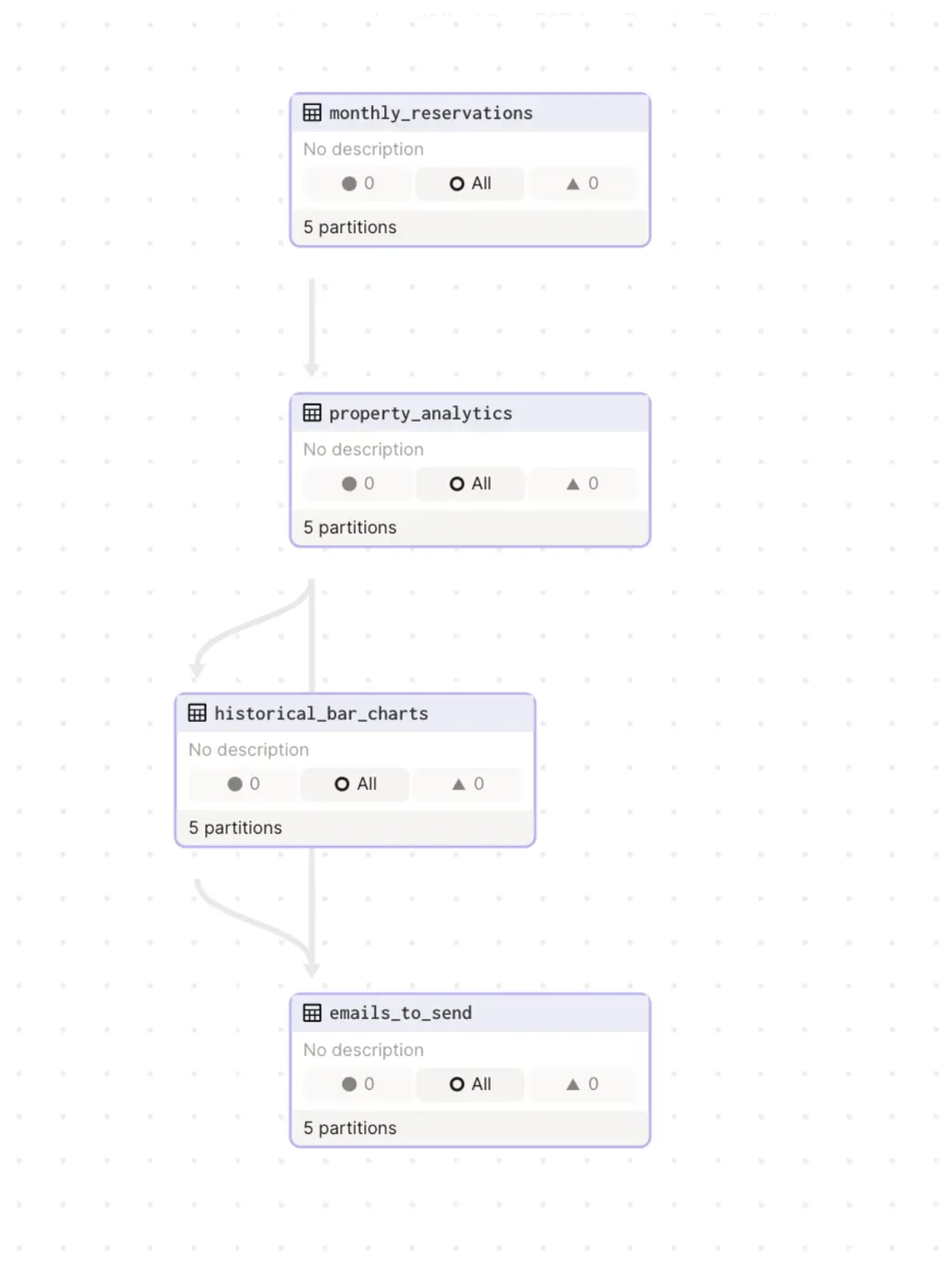
Sending the email

We’ve gathered our data and built our chart; all that’s left is sending the emails to various hosts. This step doesn’t require another asset, because it isn’t creating any output record. Instead, we need to take the assets we’ve created and do something with them, which is exactly why jobs exist.

We’ll create a job to wrap our assets, and then add an op to take the emails_to_send data and send the emails. Wrapping all of our work thus far in a single job creates a single unit of work that can be executed, scheduled, and monitored at once.

# assets.py
from dagster import job

@job(
    partitions_def=monthly_partition_def,
)
def send_emails_job():
    send_emails(emails_to_send.to_source_asset())

Like the assets in the job, the job has the monthly partition. This allows the entire job to be partitioned as a unit. The call to emails_to_send.to_source_asset() exposes the emails_to_send asset to our (currently undefined) send_emails op.

The final step is adding it to the Definition object.

# __init__.py
from .assets import send_emails_job

defs = Definitions(
    jobs=[send_emails_job],
        ...
)

Before diving into the op, we’ll need to make two resource modifications. The first change is to make our chart files readable. This involves adding a simple function to LocalFileStorage that reads a file and returns the raw bytes.

# resources.py
class LocalFileStorage(ConfigurableResource):
      ...

    def read(self, filename):
        with open(f"{self.dir}/{filename}", "rb") as image_file:
            return image_file.read()

Our second resource change is a bit more complex. We need a way to send emails, without adding that code directly to our op. A simple EmailService wraps EmailClient, which is fake but modeled on a real world commercial email service’s SDK.

# resources.py
class EmailService(ConfigurableResource):
    template_id: int
    sender_email: str
    server_token: str
    _client: EmailClient = PrivateAttr()

    def setup_for_execution(self, context) -> None:
        self._client = EmailClient(server_token=self.server_token)

    def send(self, recipient_email, template, attachments):
        self._client.send(
            sender_email=self.sender_email,
            recipient_email=recipient_email,
            template_id=self.template_id,
            template=template,
            attachments=attachments,
        )

Like every other resource, we need to add it to our Definitions object.

# __init__.py

from dagster import EnvVar
from .resources import EmailService

defs = Definitions(
        ...
    resources={
        ...
        "email_service": EmailService(
            template_id=EnvVar("EMAIL_TEMPLATE_ID"),
            sender_email=EnvVar("EMAIL_SENDER_EMAIL"),
            server_token=EnvVar("EMAIL_SERVER_TOKEN"),
        ),
    },
)

Because this configuration involves a private token, we’ll follow good security practices by setting the value as a configurable environment variable.

We’ve now covered all the necessary dependencies to look at the send_emails op.

# assets.py
@op
def send_emails(
    context: AssetExecutionContext,
    emails: pd.DataFrame,
    email_service: EmailService,
    image_storage: LocalFileStorage,
) -> None:
    bounds = context.partition_time_window
    filtered_df = emails[
        (emails["month_end"] > bounds.start) & (emails["month_end"] <= bounds.end)
    ]
    for _, row in filtered_df.iterrows():
        encoded_string = base64.b64encode(
            image_storage.read(row["total_revenue_chart"])
        ).decode()
        email_service.send(
            row["email"],
            template={
                "name": row["name"],
                "revenue": row["total_revenue"],
            },
            attachments=[
                {
                    "Name": row["total_revenue_chart"],
                    "Content": encoded_string,
                    "ContentType": "image/png",
                    "ContentID": f"cid:{row['total_revenue_chart']}",
                }
            ],
        )

Ops aren’t partitioned (since they don’t materialize data), but the job’s partition bounds are still accessible via the AssetExecutionContext object, allowing us to filter the emails DataFrame (which is the output of the prior call to emails_to_send.to_source_asset() in the job).

We can then iterate over the filtered results and send the email. The call to image_storage.read returns raw bytes, which are then encoded into a base 64 string.

Scheduling the job

The final step is to take this job and make sure it runs automatically every month. We’ll do this by defining a schedule.

# __init__.py

from dagster import ScheduleDefinition
from .assets import send_emails_job

send_emails_schedule = ScheduleDefinition(
    job=send_emails_job,
    cron_schedule="0 0 1 * *",  # every month
)

defs = Definitions(
        ...
    schedules=[send_emails_schedule],
)

This schedule will ensure our job runs every month at midnight on the first day. We can also see the schedule in the Dagster UI and toggle on/off or test different evaluation times.

Moving our pipeline into production

It’s worth considering what changes we’d need to make to this code before moving it into production.

Data access

The monthly_reservations asset does a joined database query, which could be prohibitively expensive at a sufficient scale. An alternative may be to make multiple large queries and then merge them with Pandas, but this comes at a higher memory cost. One solution at scale is creating a read replica of the database, or relevant database tables, that pipelines can query without impacting production services.

I/O Manager

Using DuckDB as an I/O Manager works well in dev, but queries are performed in memory, so it may not be feasible at production scale. An alternative is to use a production data platform as an I/O Manager. Because the architecture is pluggable, this is easy to do by creating a new resource and replacing the current one in the Definition object.

As detailed in the post “Poor Man’s Data Lake with MotherDuck" you can easily port this local project to MotherDuck, the brand new DuckDB serverless analytics platform. This would be a simple change from:

database_io_manager = DuckDBPandasIOManager(database="myvacation.duckdb", schema="main")

to

database_io_manager = DuckDBPandasIOManager(database="md:myvacation?motherduck_token={...}", schema="main")

Alternatively, you can plug into a platform like Snowflake or Databricks.

Fanning out or multi-partitioning

We create images and send emails by iterating over a large number of results. This increases the risk of a mid-execution failure that may force a lot of rework. It also means we’re working on large amounts of data at once, which could lead to memory problems. We could mitigate this by fanning out those iterations to ops that create a single chart, for example.

We’re partitioning solely on time (per month), but we could also do a multi-partition to work on smaller blocks of data at once. For example, we could partition on both time and geographic submarkets. A single partition then would represent a few thousand properties at most and would be much more manageable.

Error handling, logging, and testing

Good engineering practices go a long way, and Dagster has built-in support to simplify these. Ideally, each asset would have error handling (with retries, if appropriate) and context-specific logging that surfaces useful data regardless if asset/job succeeded or failed. Finally, all these Pandas calls are a recipe for tricky bugs that are easy to miss. Solid testing, and the designs needed to enable good testing, are essential if you were to take this into production.

We're always happy to hear your feedback, so please reach out to us! If you have any questions, ask them in the Dagster community Slack (join here!) or start a Github discussion. If you run into any bugs, let us know with a Github issue. And if you're interested in working with us, check out our open roles!

Follow us:

Sign up for our newsletter

Subscribe to the RSS feed

Star us on GitHub

Follow us on Twitter

Subscribe to our YouTube Channel