Data Extrapolation

Extrapolation definition

Data Extrapolation is a statistical method used to estimate or predict values outside a known range, based on the trends or patterns identified within the available data.

An example of extrapolation in Python

Extrapolation is an important method used in machine learning, statistics, and data engineering to predict or infer values that go beyond the original observation range. But let's be aware that while extrapolation can provide insights into potential trends, it may lead to less accurate predictions due to inherent uncertainties or changes in patterns beyond the observed data range. Let's consider a simple linear regression example with extrapolation. Here's a Python script which performs extrapolation using Scikit-Learn's linear regression. Please note that you need to have the necessary Python libraries installed in your Python environment to run this code.

import numpy as np
import matplotlib.pyplot as plt
from sklearn.linear_model import LinearRegression

# Set a random seed for reproducibility
np.random.seed(42)

# Generate some synthetic data
X = np.array(sorted(list(range(5))*20)) + np.random.normal(size=100, scale=0.5)
y = X + np.random.normal(size=100, scale=1)

# Reshape X to a 2D array
X = X.reshape(-1,1)

# Create and train the model
model = LinearRegression()
model.fit(X, y)

# Generate some future points for extrapolation
X_future = np.array(range(-2, 10)).reshape(-1, 1)

# Predict their corresponding y values
y_future = model.predict(X_future)

# Plot the original data
plt.scatter(X, y, color = "blue")

# Plot the line of best fit
plt.plot(X_future, y_future, color = "red")

# Plot the extrapolated points
plt.scatter(X_future, y_future, color = "green")

# Set title
plt.title('Linear Regression Extrapolation')

# Show the plot
plt.show()

In this script, we first generate some synthetic data, which we reshape to 2D so it can be used in the LinearRegression model. We then train the model on this data.

We generate some future X values (from -2 to 9, which goes beyond our original X values from roughly 0 to 5). We then use the model to predict what the y values for these X values will be, which is the extrapolation.

The plot shows the original data (blue dots), the line of best fit (red line), and the extrapolated points (green dots).

As you can see, the model has extrapolated the trend from the original data to the future data.

Remember, extrapolation can lead to less accurate predictions, because it's assuming that the current trend (which is derived from existing data) will continue in the future. This may not always be the case in real-world situations.

ML Extrapolation

The example above is quite basic and shows a linear model. Phillip Isola shared this interesting non-linear example of extrapolation in ML.

Phillip says:

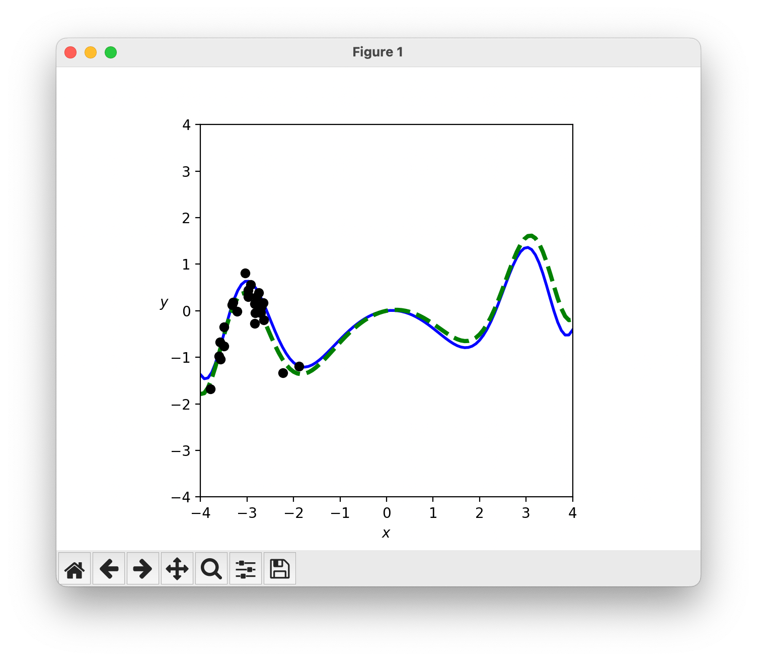
A simple, fun example to refute the common story that ML can interpolate but not extrapolate: Black dots are training points. Green curve is true data generating function. Blue curve is best fit. Notice how it correctly predicts far outside the training distribution!

You will find the code below and Phillip shared the repo here.

import numpy as np
import matplotlib.pyplot as plt

def mk_data(true_theta, noise_sd, N_data_points, data_mean, data_sd):
  data_x = np.expand_dims(np.random.randn(N_data_points)*data_sd + data_mean,axis=1)
  data_y = np.zeros(data_x.shape)
  for k in range(data_y.shape[0]):
    data_y[k,0] = np.expand_dims(np.array([f(data_x[k,0],true_theta)]),axis=1) + np.random.randn(1)*noise_sd
  data = np.concatenate([data_x,data_y],axis=1)
  return data

def mk_loss_map(data,f):
  theta_min = -2
  theta_max = 2
  [xx,yy] = np.meshgrid(np.linspace(theta_min,theta_max,101), np.linspace(theta_min,theta_max,101))

  data_fit_loss = np.zeros(xx.shape)

  for i in range(xx.shape[0]):
    for j in range(yy.shape[1]):
      theta = np.concatenate([xx[[i],j],yy[[i],j]],axis=0)
      for k in range(data.shape[0]):
        data_fit_loss[i,j] += loss(f(data[k,0], theta),data[k,1])
  data_fit_loss /= data.shape[0]

  return data_fit_loss, xx, yy

def get_best_theta(J,xx,yy):
  best_theta_idx = np.unravel_index(J.argmin(), J.shape)
  best_theta = np.concatenate([xx[[best_theta_idx[0]],best_theta_idx[1]], yy[[best_theta_idx[0]],best_theta_idx[1]]], axis=0)
  return best_theta

def mk_plot(J,data,true_theta,best_theta):

  u = 4
  xx = np.linspace(-u,u,101)
  plt.plot(xx,f(xx,best_theta),c='b',linewidth=2,zorder=1)
  plt.plot(xx,f(xx,true_theta),'--',c='g',linewidth=3,zorder=2)
  plt.scatter(data[:,0],data[:,1],c='k',zorder=3)
  plt.gca().set_xlim(-u,u)
  plt.gca().set_ylim(-u,u)
  plt.gca().set_aspect('equal')
  plt.gca().set_xlabel('$x$')
  plt.gca().set_ylabel('$y$',rotation=0)

def mk_fit(true_theta, noise_sd, N_data_points, data_mean, data_sd):
  data = mk_data(true_theta, noise_sd, N_data_points, data_mean, data_sd)
  J, xx, yy = mk_loss_map(data,f)
  best_theta = get_best_theta(J, xx, yy)
  return J, best_theta, data

def f(x,theta):
  y = np.sin(theta[1]*x**2) + theta[0]*x
  return y

def loss(x,y):
  return np.abs(x-y)**0.25


seed = 4
np.random.seed(seed)

true_theta = np.array([0.2,-0.5])
noise_sd = 0.2

data_mean = -3
data_sd = 0.5
N_data_points = 25
J, best_theta, data = mk_fit(true_theta, noise_sd, N_data_points, data_mean, data_sd)
mk_plot(J, data, true_theta, best_theta)

# Show the plot
plt.show()