Normality Testing

Normality testing definition:

Normality testing is a statistical technique used to determine if a given sample or population data follows a normal distribution. A normal distribution, also known as a Gaussian distribution, is a bell-shaped curve that is symmetric around the mean. Normality testing comes in handy if you want to test the assumption that your data follows a normal distribution.

There are several methods and libraries/functions for normality testing when working in Python, the three most used ones being:

• Shapiro-Wilk test: This test calculates a W statistic that tests the null hypothesis that the data was drawn from a normal distribution. The test returns a p-value which can be used to determine if the null hypothesis can be rejected or not.
• Kolmogorov-Smirnov test: This test calculates a D statistic that measures the distance between the empirical distribution function of the sample and the cumulative distribution function of the normal distribution. The test returns a p-value which can be used to determine if the null hypothesis can be rejected or not.
• Anderson-Darling test: This test calculates an A2 statistic that measures the distance between the sample and the theoretical distribution. The test returns a critical value which can be compared with the A2 statistic to determine if the null hypothesis can be rejected or not.

Normality testing example using Python:

Please note that you need to have the necessary Python libraries installed in your Python environment to run the following code examples.

Shapiro-Wilk test

Here is a practical example of how to perform a normality test using the Shapiro-Wilk test in Python:

from scipy import stats
import numpy as np

# Generate a random sample of 1000 numbers from a normal distribution
sample = np.random.normal(loc=0, scale=1, size=1000)

# Perform Shapiro-Wilk test on the sample
shapiro_test = stats.shapiro(sample)

# Print the test statistics and the p-value
print('Shapiro-Wilk test statistics: ', shapiro_test[0])
print('Shapiro-Wilk test p-value: ', shapiro_test[1])

In this example, we generated a random sample of 1000 numbers from a normal distribution and then performed the Shapiro-Wilk test on the sample. The stats.shapiro() function from the scipy library is used to perform the test, and it returns two values: the test statistic and the p-value. Since the numbers are random, the output will vary, but will look something like this:

Shapiro-Wilk test statistics:  0.9981188774108887
Shapiro-Wilk test p-value:  0.33603352308273315

The test statistic is used to determine if the sample follows a normal distribution or not. If the p-value is less than the significance level (usually 0.05), then we reject the null hypothesis and conclude that the sample does not follow a normal distribution. If the p-value is greater than the significance level, then we fail to reject the null hypothesis and conclude that the sample follows a normal distribution.

Kolmogorov-Smirnov test

The Kolmogorov-Smirnov test (K-S test) is a type of non-parametric test that you can use to compare a sample with a reference probability distribution (one-sample K-S test), or to compare two samples (two-sample K-S test). It is a method to identify if your data significantly deviates from a specified distribution.

Here's a simple Python program for K-S test using the SciPy library, which is a library for scientific computations in Python. For this example, we'll use the one-sample K-S test to test if a given sample follows a normal distribution.

First, you will need to install the necessary libraries, numpy, scipy and matplotlib. We also provide a full list of Python libraries with install commands here. Either way, for this example can do this using pip:

pip install numpy scipy matplotlib

Here is the Python code:

import numpy as np
from scipy import stats
import matplotlib.pyplot as plt

# generate a gaussian random variable sample
np.random.seed(0)  # for reproducibility
sample_size = 1000
sample = np.random.normal(loc=0, scale=1, size=sample_size)

# perform Kolmogorov-Smirnov test
D, p_value = stats.kstest(sample, 'norm')

print(f'K-S statistic: {D}')
print(f'p-value: {p_value}')

# visual check
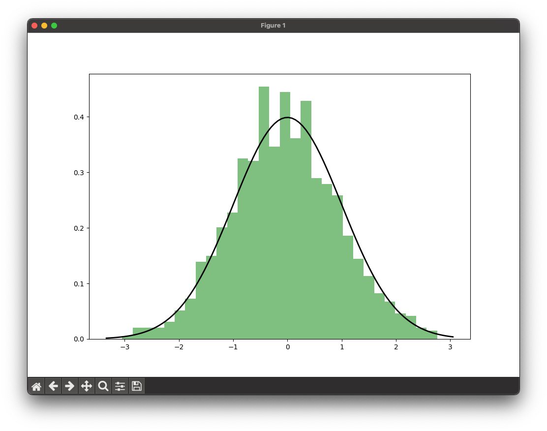
plt.figure(figsize=(10, 7))
plt.hist(sample, bins=30, density=True, alpha=0.5, color='g')
xmin, xmax = plt.xlim()
x = np.linspace(xmin, xmax, 100)
p = stats.norm.pdf(x, 0, 1)
plt.plot(x, p, 'k', linewidth=2)
plt.show()

This script first generates a sample of 1000 data points from a normal distribution with mean 0 and standard deviation 1. Then it performs the K-S test using the kstest function from the scipy.stats module, comparing the sample to a standard normal distribution. The test returns the K-S statistic D and the p-value of the test.

If the K-S statistic is small or the p-value is high (greater than the significance level, say 0.05), then we cannot reject the hypothesis that the distributions of the two samples are the same. Otherwise, we reject the hypothesis and conclude that the distributions are different.

Finally, a histogram of the sample and the PDF (probability density function) of the standard normal distribution are plotted.

As our sample is randomly generated, we cannot predict your output, but it will look something like this:

K-S statistic: 0.03737519429804048
p-value: 0.11930823166569182